
Part 1 — The Old World: Data vs Model Parallel
Before ZeRO, this is how we scaled AI — and where it broke.

The last decade of deep learning has been a balancing act between model complexity and hardware limits.
Each time we added parameters, we collided with memory ceilings, bandwidth bottlenecks, or communication delays.
To push past those limits, engineers turned to parallelism — splitting either the data or the model across GPUs.
At first, that was enough.
But as models grew from millions to billions (and now trillions) of parameters, those early strategies began to crack.
🧩 The Single-GPU Baseline
Let’s start with the simplest case — a single GPU training a model.
Each iteration has four key steps:
Forward pass: compute predictions from input data.
Loss calculation: measure how far predictions are from targets.
Backward pass: compute gradients (∂L/∂W) using backpropagation.
Optimizer step: update weights (W ← W − η · ∂L/∂W).
Everything — parameters, gradients, optimizer states — lives in one GPU’s memory.
This works perfectly fine… until the model doesn’t fit in memory -VRAM, anymore.
⚙️ Data Parallelism — Many Copies, Different Data
The simplest form of scaling is to replicate the model across multiple GPUs.
Each GPU gets a different mini-batch of data but an identical copy of the model.
During training:
Each GPU runs its forward and backward passes independently.
Gradients are calculated locally.
At the end of the iteration, all GPUs average their gradients using a communication operation called all-reduce.
Each GPU updates its weights — which remain synchronized across all devices.
💡 What It Looks Like
Imagine four GPUs, each processing a unique set of training samples.
They all hold the same model, compute gradients, then synchronize.
[GPU1] ─┐
[GPU2] ─┤──►  all-reduce  ─►  averaged gradients
[GPU3] ─┤
[GPU4] ─┘
After this, all GPUs have identical weights, ensuring consistent model state across devices.
✅ Advantages
Simple: minimal code changes from single-GPU training.
Scalable: easily add GPUs for larger batch sizes.
Synchronous: deterministic updates and convergence.
❌ Limitations
Memory waste: every GPU stores the same parameters, gradients, and optimizer states.
Example: a 10B-parameter model (in FP16) requires 20 GB just for weights, and 60–80 GB once optimizer states are included.
With 8 GPUs, that’s 8× redundancy.
Synchronization cost: gradient averaging (all-reduce) becomes expensive across nodes.
No help for large models: if the model doesn’t fit on one GPU, replication won’t solve it.
🔧 In PyTorch Implementation
import torch.distributed as dist

# Example: average gradients across all GPUs
dist.all_reduce(tensor, op=dist.ReduceOp.SUM)
tensor /= dist.get_world_size()
This is the core of traditional Data Parallel training.
🧠 Model Parallelism — Splitting the Model Itself
When a model can’t fit on one GPU, parameters are partitioned instead of replicating them.
Each GPU holds a different slice of the model.
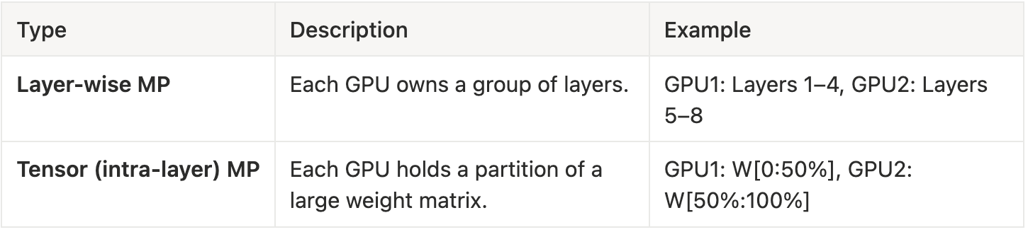
There are two main styles:
During training:
Forward activations flow through the GPUs in sequence.
Backpropagation flows in reverse order.
This keeps total memory per GPU low but increases communication dramatically.
💡 Visual Example (Layer-wise MP)
Input → [GPU1: Layers 1–4] → [GPU2: Layers 5–8] → Output
In backpropagation:
Output Gradients → [GPU2] → [GPU1] → Parameter Updates
Each stage depends on data from the previous one — no GPU can move forward until the prior GPU is done. In other words communication between GPUs happens every layer — not just once per iteration.
🛰️ Communication in Model Parallelism
1. Layer-wise (Pipeline) Parallelism
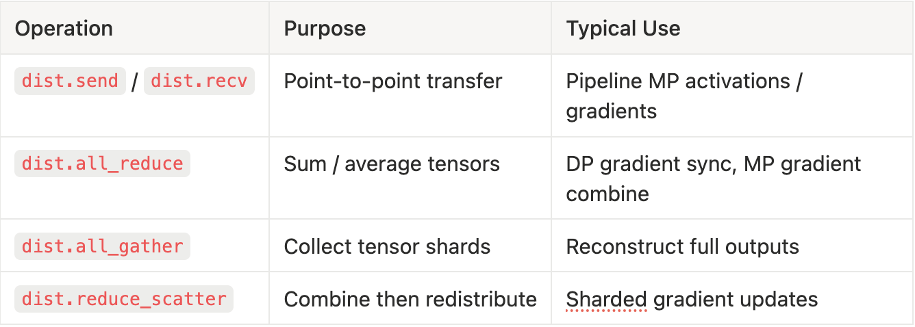
Each GPU sends activations forward and gradients backward.
Implemented with point-to-point ops:
dist.send(tensor=activations, dst=next_rank)
dist.recv(tensor=grads, src=prev_rank)
Transfer volume ≈ (batch × hidden × dtype_bytes).
E.g. batch 16 × 8k activations × 2 bytes = ~256 kB per micro-batch.
2. Tensor (Intra-layer) Parallelism
Each GPU holds a shard of the weight matrix WWW.
Forward pass: partial outputs computed locally → all-gather to assemble Y.
Backward pass: gradients reduced across GPUs → reduce-scatter or all-reduce.
# Forward: gather partial outputs
dist.all_gather(list_of_tensors, partial_output)

# Backward: combine gradients
dist.all_reduce(grad_tensor, op=dist.ReduceOp.SUM)
Communication per layer ≈ 2 × tensor_size (one forward, one backward).
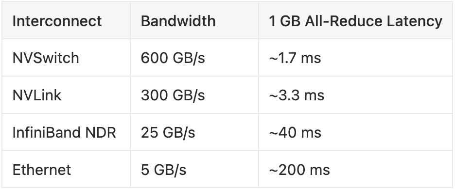
3. Summary of Collectives
Communication time ≈ α log N + β S / B
where α = latency, β = bytes, B = bandwidth, N = #GPUs.
✅ Advantages
Memory-efficient: each GPU stores only part of the model.
Enables massive models: used in GPT-3 and beyond.
❌ Limitations
Communication-heavy: activations and gradients are passed between GPUs at every layer.
Pipeline bubbles: idle GPUs while waiting for upstream/downstream layers.
Complex orchestration: load balancing and synchronization become tricky.
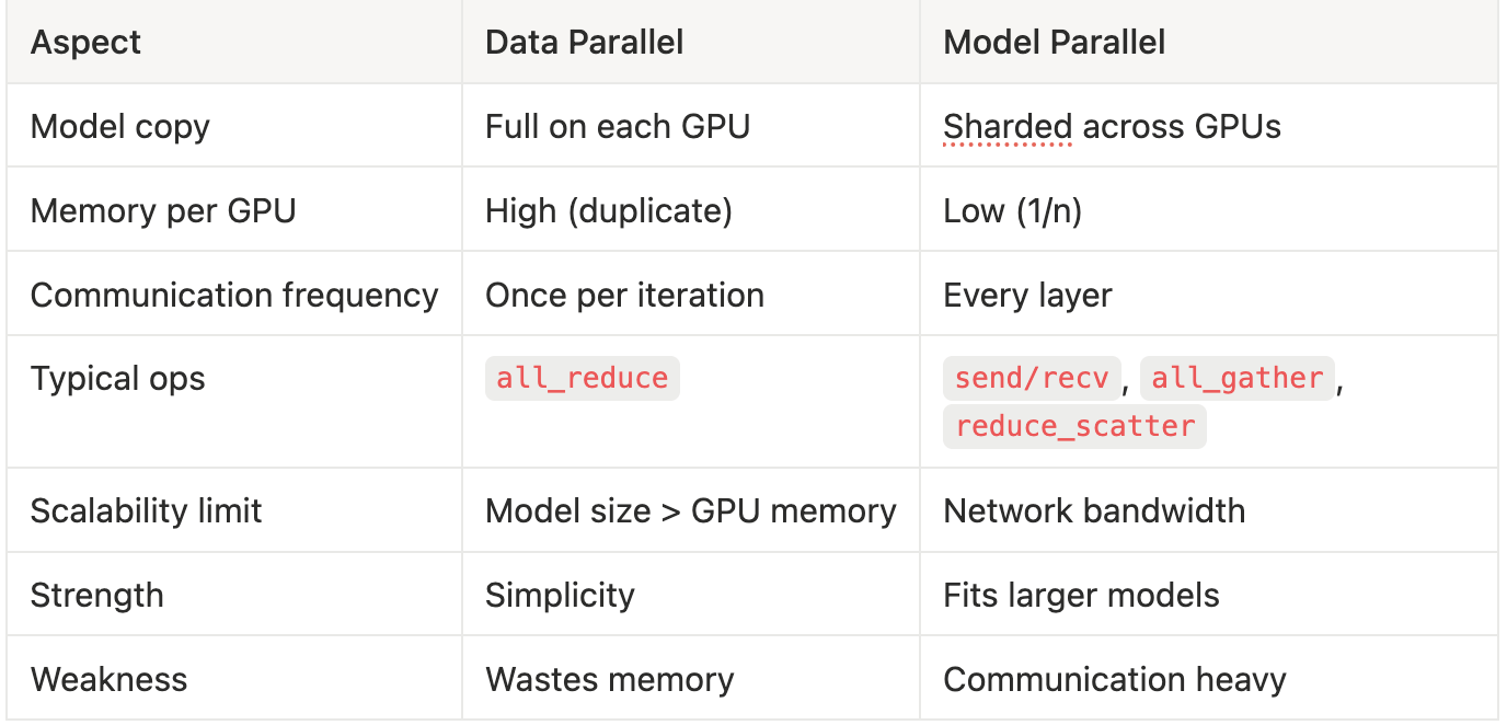
⚖️ Comparing the Two
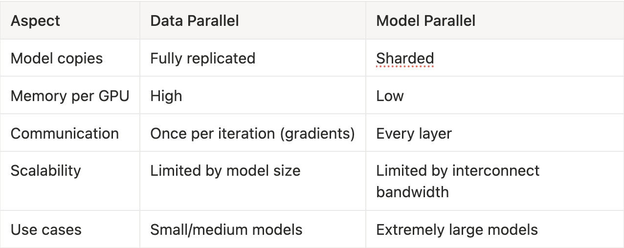
Each method solves one problem but amplifies another.
Data Parallelism is easy but redundant.
Model Parallelism is efficient but complex and communication-bound.
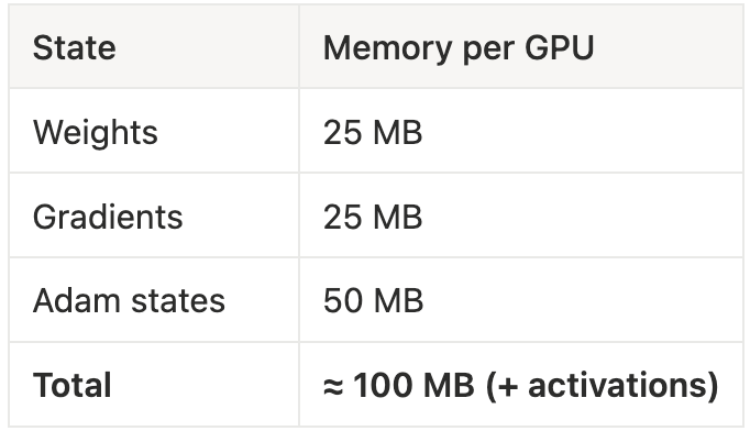
🧮 Memory and Processing Estimates
Example: 100 M-parameter model (FP16)
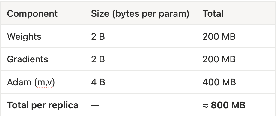
Under Data Parallelism
Each GPU stores all states → 800 MB × #GPUs.
8 GPUs = 6.4 GB duplicated.
For billion-parameter models, this scales to terabytes.
Under Model Parallelism (n = 8)
Memory saves ≈ 1/n, but each layer now triggers two collectives.
For a 96-layer transformer, ≈ 19 GB of data may move per iteration.
⚡ Compute vs Communication Trade-off
Let:
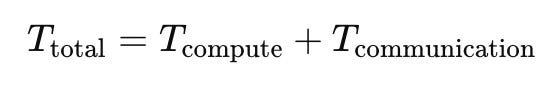
Approximate communication time:
As models grow, T(communication)can exceed
T(compute) — scaling → stalls even with more GPUs.
⚖️ Data vs Model Parallel Summary
💥 The Breaking Point
As model sizes passed hundreds of billions of parameters, even combining these approaches wasn’t enough.
With Data Parallel + Model Parallel hybrid setups, teams faced:
GPUs sitting idle waiting on communication.
Memory exhaustion from optimizer states.
Gigantic gradient synchronization delays across nodes.
At this scale, every inefficiency — every duplicated tensor, every redundant state — becomes a bottleneck.
I have breakdown the memory usage for Transformer in my blog in details to explain the math:
That’s where ZeRO (Zero Redundancy Optimizer) entered the picture:
a way to keep the math of data parallelism but eliminate its memory waste —
sharding not just the model, but also the optimizer states and gradients across GPUs.
🧭 Takeaway
Before ZeRO, parallelism was a tug-of-war:
Data Parallelism wasted memory to stay simple.
Model Parallelism saved memory but cost time and coordination.
ZeRO found a middle ground — making data parallelism memory-efficient without changing its elegant simplicity.
That’s what we’ll unpack in Part 2: ZeRO-DP — Partition, Don’t Replicate.
About the Author
Sheetal Gotpagar — Engineering Leader | AI Infrastructure Strategist
The ZeRO Playbook is my ongoing series on engineering efficiency at scale — inspired by Microsoft’s ZeRO, evolved through real-world systems design.
That breakdown of data parallelism was super clear. Makes you think about the network overhead for all-reduce with massiv models, no?